
I have spent enough time inside spreadsheets to know that duplicates are rarely harmless. They hide in sales reports, student rosters, payroll exports, and CRM downloads. They distort totals, inflate counts, and quietly undermine decisions. That is why knowing how to highlight duplicates in Excel is more than a cosmetic trick. It is a safeguard.
The fastest way to highlight duplicates in Excel is through Home → Conditional Formatting → Highlight Cells Rules → Duplicate Values. Select your range, choose a format, and Excel instantly marks repeated entries, including the first occurrence. For more control, especially if you want to exclude the first instance or highlight entire rows, use a formula such as =COUNTIF($A$2:$A2,$A2)>1 inside a New Rule. For multi-column matches, COUNTIFS provides precise row level detection. And if you need to compare across sheets, reference another sheet directly inside your formula.
Microsoft Excel, first released in 1985 for Macintosh and later for Windows in 1987, has evolved into one of the most widely used analytical tools in the world. According to Microsoft’s 2023 reporting, Microsoft 365 has hundreds of millions of commercial users globally. Within that ecosystem, Excel remains central.
Duplicates are not just formatting concerns. They are data integrity issues. Highlighting them is often the first step toward cleaning, validating, and trusting your information.
Why Duplicates Matter More Than You Think

Duplicate entries distort reporting. A duplicated invoice number may inflate revenue totals. A repeated email address in a marketing list can skew campaign metrics. A duplicated ID in a research dataset may invalidate conclusions.
Harvard Business Review has reported extensively on the cost of poor data quality, noting that flawed data leads to flawed decisions across industries. Even small duplication errors can cascade into larger analytical problems.
Excel’s Conditional Formatting feature provides immediate visual feedback. Rather than manually scanning rows, the software flags repeated values automatically. – how to highlight duplicates in excel.
Data expert and author Jordan Goldmeier has written that spreadsheets are powerful but “only as reliable as the structure behind them.” Highlighting duplicates is part of building that structure.
The ability to detect repetition visually turns a spreadsheet from a passive grid into an active diagnostic tool.
Read: ChromiumFX: Embedding Chromium in .NET Apps
The Basic Method: Highlight All Duplicate Values

For quick results, Excel offers a built in duplicate detection rule.
Steps:
- Select your data range, for example A1:A100.
- Go to Home → Conditional Formatting → Highlight Cells Rules → Duplicate Values.
- Choose a formatting style such as light red fill with dark red text.
- Click OK.
Excel highlights every occurrence of a repeated value, including the first one.
This method works in Excel for Microsoft 365, Excel 2021, Excel 2019, and earlier versions. It is ideal for fast audits when you need a broad overview.
However, this approach treats all repeated entries equally. It does not distinguish between original and subsequent duplicates. In many workflows, especially reconciliation tasks, users prefer to highlight only the extra occurrences.
That is where formulas provide deeper control.
Advanced Method: Excluding the First Occurrence
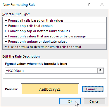
To highlight only repeated entries beyond the first instance, use a formula based rule.
- Select your data range starting from the first data row, for example A2:A100.
- Go to Home → Conditional Formatting → New Rule.
- Choose “Use a formula to determine which cells to format.”
- Enter:
=COUNTIF($A$2:$A2,$A2)>1
This formula counts how many times the current value has appeared from the top of the list down to the current row. If the count exceeds one, Excel highlights it.
The dollar sign locks the column reference while allowing the row to adjust dynamically.
| Formula | Result |
|---|---|
>1 | Highlights duplicates excluding first |
>=1 | Highlights all including first |
>2 | Highlights triplicates and beyond |
This technique is essential for auditing lists where the first record is legitimate and subsequent entries require attention.
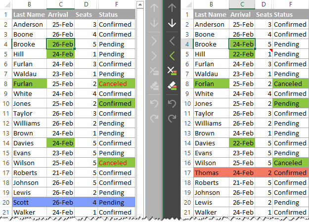
Highlighting Entire Duplicate Rows

Often, duplicates span multiple columns, such as first name and last name combinations or product ID and order date pairs.
To highlight entire rows:
- Select the full dataset, for example A2:D100.
- Create a new Conditional Formatting rule.
- Enter:
=COUNTIFS($A$2:$A$100,$A2,$B$2:$B$100,$B2)>1
This checks whether the combination of columns A and B repeats anywhere in the range.
Extend the formula with additional column pairs as needed.
Excel evaluates each row holistically rather than cell by cell. This approach prevents false positives when individual cells repeat but row combinations differ.
For structured datasets such as transaction logs or HR exports, row level detection ensures meaningful duplication analysis.
Highlighting Duplicates Across Multiple Columns Using a Helper Column

In wide datasets, writing long COUNTIFS formulas can become unwieldy. A helper column simplifies the process.
In a new column, combine relevant fields:
=A2&"|"&B2&"|"&C2
The pipe character acts as a separator, preventing accidental matches such as AB equaling A and B concatenated differently.
Apply Conditional Formatting with:
=COUNTIF($E$2:$E$100,$E2)>1
This method centralizes duplication logic in a single column.
Microsoft’s Excel documentation highlights concatenation as a flexible data preparation technique. In complex audits, helper columns provide clarity and maintainability.
They also make it easier to sort or filter duplicates without rewriting formatting rules.
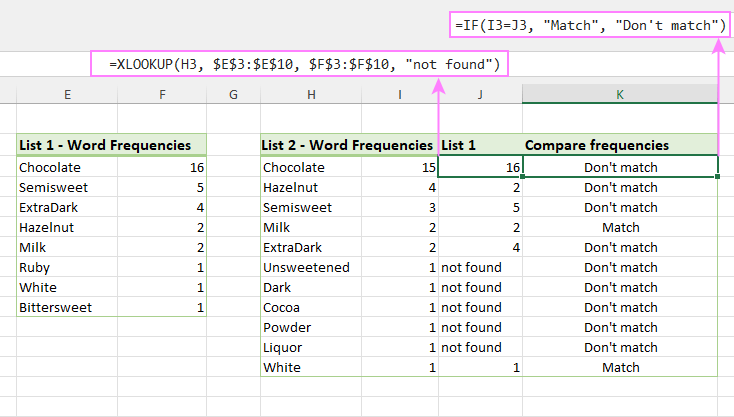
Comparing Duplicates Across Two Sheets
Cross sheet duplication checks are common when reconciling exports from different systems.
On Sheet1:
Select A2:A100 and use:
=COUNTIF(Sheet2!$A$2:$A$100,$A2)>0
Excel highlights values in Sheet1 that appear in Sheet2.
For row level comparison across columns A and B:
=COUNTIFS(Sheet2!$A$2:$A$100,$A2,Sheet2!$B$2:$B$100,$B2)>0
If a sheet name contains spaces, wrap it in single quotes, such as 'Sales 2024'!$A$2:$A$100.
This method is especially useful in financial reconciliation, where transactions must match between systems.
Highlighting Triplicates or Higher Multiples
Sometimes duplicates are acceptable, but three or more repetitions signal a problem.
Modify your formula:
=COUNTIF($A$2:$A$100,$A2)>2
This highlights values appearing at least three times.
For multiple columns:
=COUNTIFS($A$2:$A$100,$A2,$B$2:$B$100,$B2)>2
These thresholds allow nuanced data validation.
| Threshold | Meaning |
|---|---|
>1 | Duplicates |
>2 | Triplicates or more |
>3 | Four or more instances |
Fine tuning thresholds transforms Conditional Formatting into a data auditing engine rather than a simple coloring tool.
Removing Duplicates After Highlighting
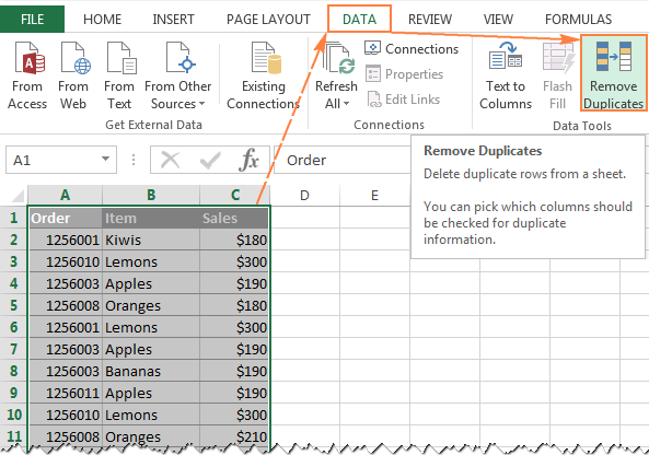
Highlighting does not delete data. It only identifies it.
To remove duplicates:
- Select your data.
- Go to Data → Remove Duplicates.
- Choose relevant columns.
- Click OK.
Excel retains the first instance and deletes subsequent duplicates.
For cautious workflows, filter by color first to inspect highlighted rows. Then delete manually.
Always create a backup copy before removal. Data deletion is permanent unless undone immediately.
Excel’s Remove Duplicates tool was introduced in Excel 2007 as part of Microsoft’s broader push toward data management capabilities.
Highlighting first ensures informed decisions before deletion.
Managing and Clearing Formatting Rules
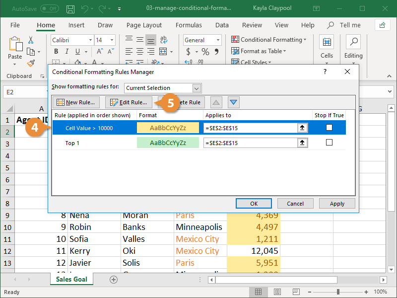
Conditional Formatting rules accumulate over time. Conflicting rules may override each other.
To manage rules:
Home → Conditional Formatting → Manage Rules.
To remove:
Home → Conditional Formatting → Clear Rules → Clear Rules from Selected Cells.
Maintaining rule hygiene prevents unexpected visual conflicts.
Spreadsheet consultant and author Mike Girvin has emphasized that transparency in formulas improves spreadsheet governance. The same applies to formatting logic.
Cluttered formatting can obscure rather than illuminate data.
Takeaways
- Use Highlight Cells Rules for fast duplicate detection.
- Use COUNTIF to exclude first occurrences.
- Use COUNTIFS for multi column row matching.
- Helper columns simplify complex duplicate logic.
- Compare across sheets with direct sheet references.
- Adjust thresholds to detect triplicates or higher multiples.
- Remove duplicates carefully after reviewing highlighted data.
Conclusion
I have come to see duplicates not as minor spreadsheet annoyances but as signals. They signal process breakdowns, import inconsistencies, and sometimes deeper data integrity issues.
Excel’s Conditional Formatting system gives users a visual language for identifying those signals. With a few formulas, you can move beyond basic duplication checks and build layered validation systems. Highlighting entire rows, comparing across sheets, filtering by color, and adjusting frequency thresholds transform a simple grid into a controlled analytical environment.
Excel has endured for nearly four decades because it balances accessibility with power. Highlighting duplicates is one of its most deceptively simple features. Used thoughtfully, it prevents reporting errors, improves trust in datasets, and safeguards decision making.
The color that appears in a cell is more than decoration. It is information asking for attention.
FAQs
1. Does highlighting duplicates delete them?
No. Conditional Formatting only marks cells visually. Use Data → Remove Duplicates to delete entries.
2. Can I highlight duplicates in Excel tables?
Yes. Select the table range and apply Conditional Formatting as usual.
3. Why is my formula not highlighting correctly?
Check absolute references with dollar signs. Incorrect locking often causes errors.
4. Can I highlight duplicates in Excel Online?
Yes. Excel for the web supports Conditional Formatting with duplicate rules.
5. How do I highlight duplicates in one column only?
Select the specific column range before applying Conditional Formatting.